Image Masking Challenge. A Kaggle Competition
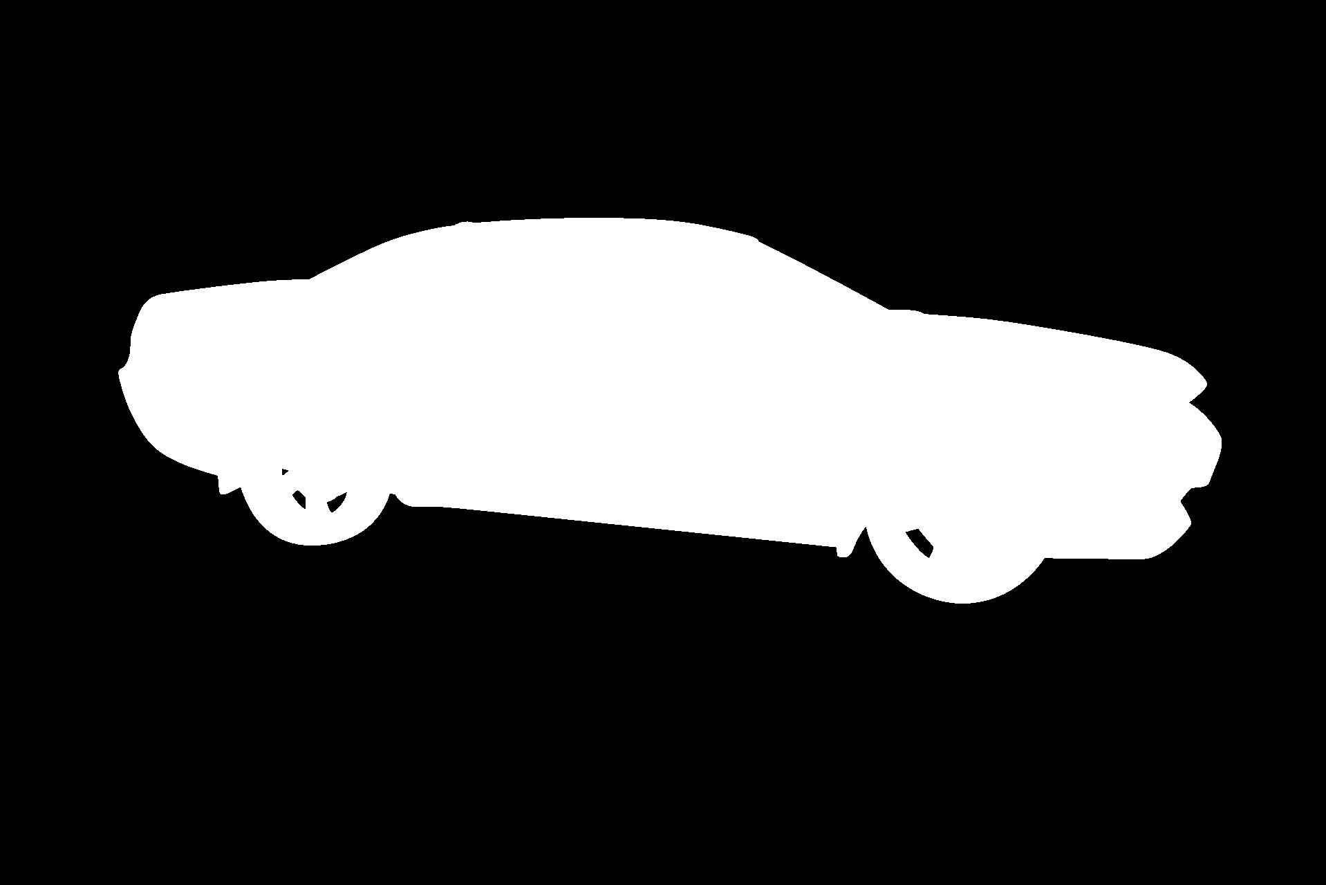
The goal of this Kaggle competition is to remove the background of a set of car pictures with a width variety of year, color and model combinations. That means, creating a mask for each photo that covers the area where the vehicle is. Using Machine Learning in this task would save a lot of time in manual photo editing.
To achieve that, a train and test dataset is provided with 5088 (404 MB) and 100064 (7.76 GB) photos respectively. For each car in the datasets, there is an image of it from 16 different angles and for each of these images (just in the training dataset), there is the mask we want to predict. These images have a resolution 1918x1280 pixels. The goal of this competition is to predict the mask for the test images.
As in many human tagged datasets, this is not fully consistent. Since the training masks have been created by humans, for instance, some of them take into account holes in the wheels or car antenna, and others don’t.

To do deal with that, this Image Segmentation problem has been approached with Neural Networks.
Neural Network Architecture
The main Neural Network Architecture used in this project is the U-net. This architecture has the state-of-the-art in Image Segmentation.
This NN is made with lots of Convolutional Layers according to an Autoencoder structure where the data is downsampled after a fixed number of layers in the encoder and upsampled in the decoder. However, unlike autoencoders, the output of each layer in the encoder is also concatenated to the input of its analog layer in the decoder. This method allows an easiest reconstruction of the NN input.
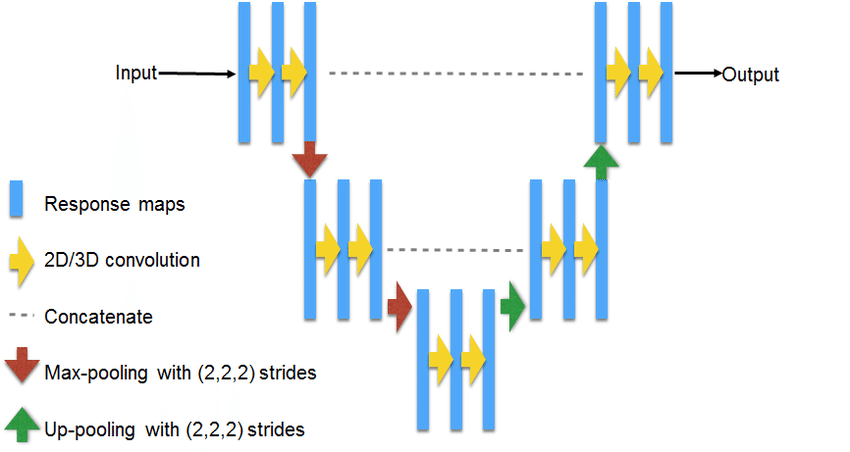
After some hyperparameter tuning, I have used an architecture where all of the layers in the encoder and decoder are made with two single Convolutional Layers and Batch Normalization to avoid overfitting. Also, each block of layers is followed by a MaxPooling layer in the encoder and preceded by an UpSampling layer in the decoder. In general terms, the tests I made show that the bigger the NN is, the better the results it achieves, but the more resources it needs. So, the final NN architecture I used has 18 Convolutional Layers, quite deep to be trained in a laptop…
Training
The score to be evaluated in this competition is the Dice Coefficient, that calculates the difference between the pixel intersection from the original and predicted masks, and the sum of the pixels from both masks. This score is a value between 0 and 1, where 1 is the best value that can be achieved.
$$Dice = \frac{2 * |X \cap Y|}{|X| + |Y|}$$
To optimize that metric, the Neural Network has been trained to reduce the Binary Cross Entropy Loss (BCE) as a normal classification problem. However, after some tests, this function was changed to another Loss Function that combines both BCE and Dice Coefficient, showing a slight improvement on the competition score. The idea of combine both metrics is to check several kinds of errors before the weights updates.
$$Loss = BCE + (1 - Dice)$$
Data Preprocessing
Another kind of parameters to tune are those related with the image preprocessing. In the first place, using RGB images shows better results than just using grayscale images, without a significant increase of the required resources.
As the training dataset is much smaller than the test dataset, one of the most successful improvements I did was to augment it by performing some image transformations. The transformations I used include data rescalation, shearing, rotation, width and height shifting, and horizontal flip. This augmentation is made on the fly on images and masks from the training dataset. With this method, the trained model is able to generalize better to fit the test data.
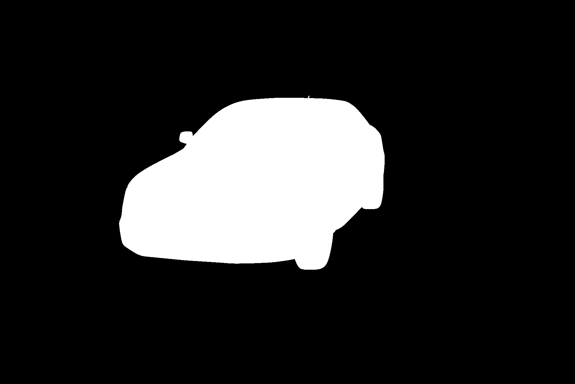
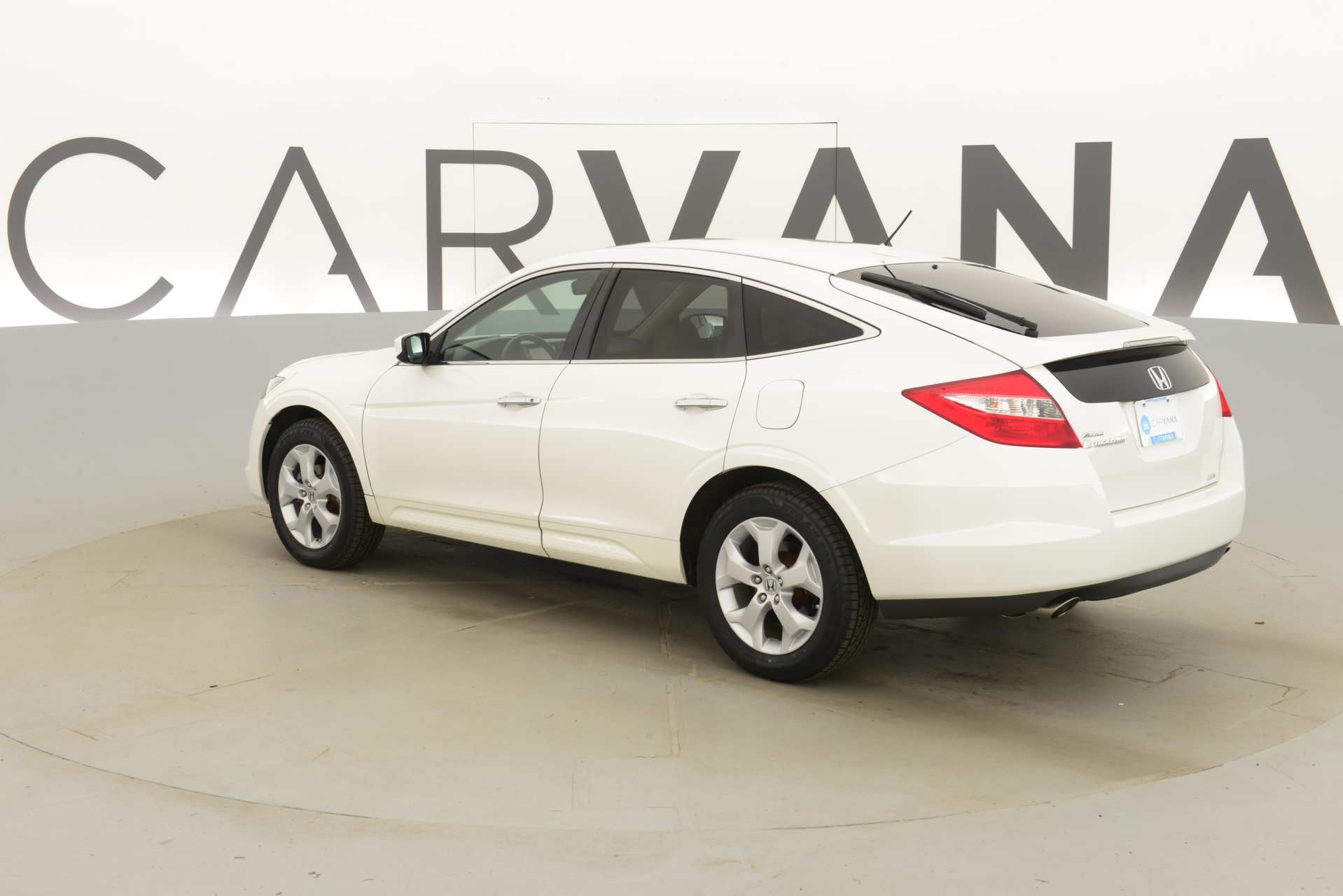
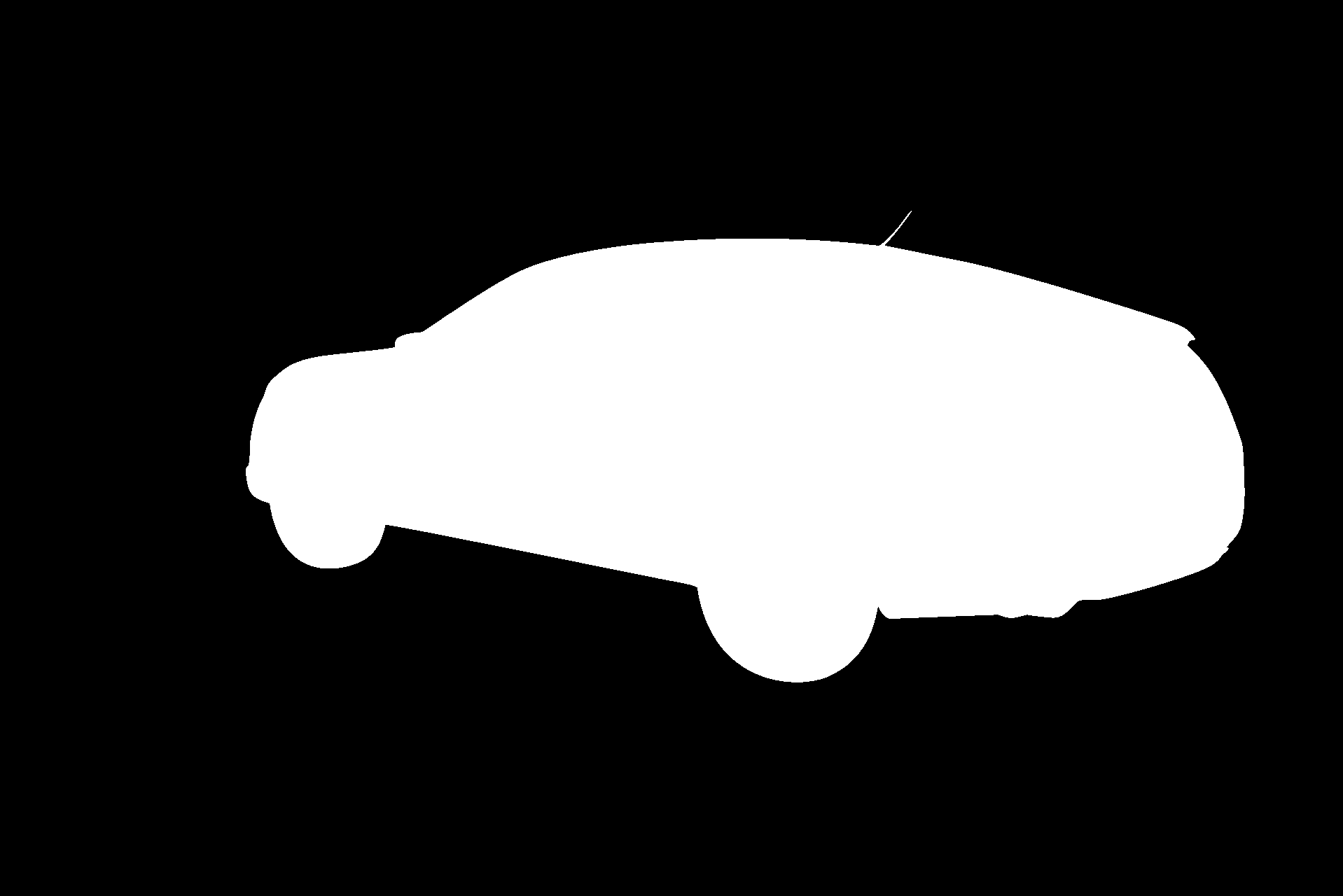
/train/original_img_5.png)
/train/original_mask_5.png)
/train/predicted_mask_5.png)
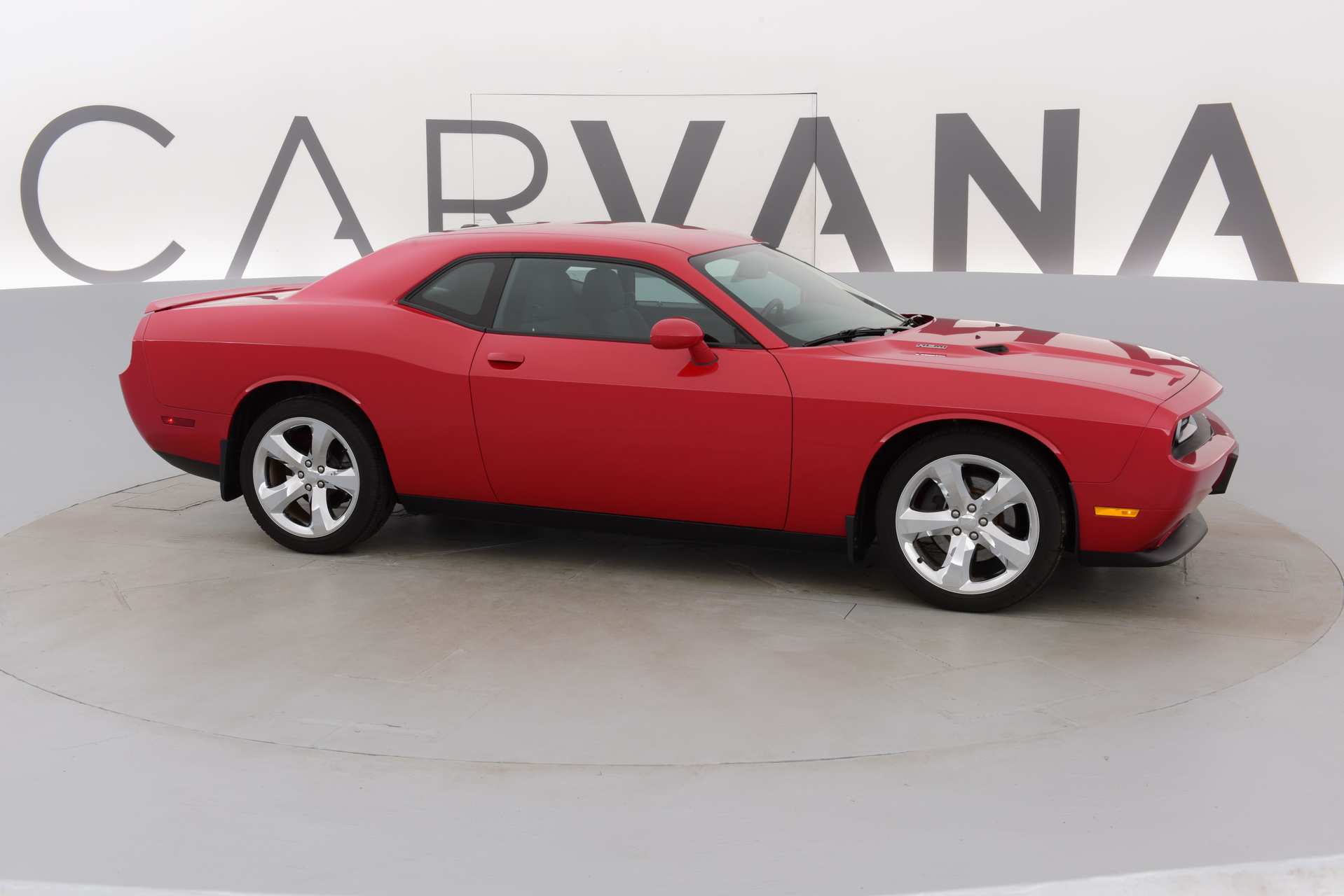
/train/original_img_2.png)
/train/original_mask_2.png)
/train/predicted_mask_2.png)
One of the most important parameter that most influences the final result is the image size. This really affects the final result and the necessary resources to process all the data. The bigger the input image is, the better the results will be, but more GPU memory will be needed. To find a tradeoff between the input size and the computing requirements, the batch size during training must be reduced, but this reduction can also affect the results.
By tuning these parameters the best score I got was with an input size of 768x768x3 and a batch size of 4. The biggest input image that my GPU can handle is 1024x1024x3 with a batch size of 1, however, this small batch size leads to a big overfitting in the predicted mask.
/val/original_img_2.png)
/val/predicted_mask_2.png)
/val/original_img_4.png)
/val/predicted_mask_4.png)
When training Neural Networks, one common technique is to split the training dataset in training and validation to check the model performance over each epoch. However, since all photos look quite similar, the test metrics (in training and validation datasets) were decreasing at the same time without a significant change. For that reason, I decided not to split the training dataset and use the full training data to train the model. Although this lead to a small improvement on the final score, this is not an action to extrapolate to other problems in Machine Learning.
Conclusions
After all the parameter tuning, the trained model is able to predict masks almost identical to the original ones. With this result, I achieved a Dice score of 0.9964 in the Private Leaderboard and a position in the 18% percentile, just only 0.0009 points of difference with the winner’s score.
/val/original_img_8.png)
/val/final_predicted_mask_8.png)
/val/original_img_3.png)
/val/final_predicted_mask_3.png)
Further work
Although the results are very accurate, there are still some improvements that could increase the final obtained score:
- The best improvement would be to use a bigger GPU that is capable to handle bigger input images and deeper models.
- Accumulate gradients before updating the weights. This can help when dealing with a small batch size.
- Stacked model. Join all the predicted masks from different models (with different parameters) to feed another model or to calculate the final mask by voting/averaging the pixels from all masks.
- Change the pairs of Convolutional Layers to Dense Blocks. In this model, the output of a Dense Block (two Convolutional Layers) is concatenated with its input and optionally with the previous Dense Blocks’ output (with the required downsampling or upsampling). This technique should avoid problems like the vanishing gradient.
- Test a training using a combination of different metrics like the Jaccard Coefficient in the Loss Function. These functions can also be used to measure the accuracy of the model instead of using the Dice Coefficient.
Full code is available in this Github repo.